graphics

As a chemist it is often useful to plot electronic orbitals.  These are used to describe the wave function of electrons in atoms or molecules.  Typically, these are output from electronic structure software in the form of a cube file, first developed by Gaussian.  These files contain volumetric data for a given orbital on a three-dimensional grid.

There exist many applications to visualize cube files, such as VMD or GaussView, but I wanted to take advantage of Mathematica‘s  capability to easily combine graphics, as well as the ability to automate the process in order to efficiently create frames for a movie.

First off, we need a function to extract the data from the cube file.  In the process, we will create the text for an XYZ file, a format also developed by Gaussian.  The function OutForm is used here to mimic the printf function found in other programming languages.

OutForm[num_?NumericQ, width_Integer, ndig_Integer, 
   OptionsPattern[]] :=
  Module[{mant, exp, val},
   {mant, exp} = MantissaExponent[num];
   mant = ToString[NumberForm[mant, {ndig, ndig}]];
   exp = If[Sign[exp] == -1, "-", "+"] <> IntegerString[exp, 10, 2];
   val = mant <> "E" <> exp;
   StringJoin@PadLeft[Characters[val], width, " "]
   ];


ReadCube[cubeFileName_?StringQ] := Module[
   {moltxt, nAtoms, lowerCorner, nx, ny, nz, xstep, ystep, zstep, 
    atoms, desc1, desc2, xyzText, cubeDat, xgrid, ygrid, zgrid, 
    dummy1, dummy2, atomicNumber, atomx, atomy, atomz, tmpString, 
    headerTxt,bohr2angstrom},
   bohr2angstrom = 0.529177249;
   moltxt = OpenRead[cubeFileName];
   desc1 = Read[moltxt, String];
   desc2 = Read[moltxt, String];
   lowerCorner = {0, 0, 0}; 
   {nAtoms, lowerCorner[[1]], lowerCorner[[2]], lowerCorner[[3]]} = 
    Read[moltxt, String] // ImportString[#, "Table"][[1]] &;
   xyzText = ToString[nAtoms] <> "\n";
   xyzText = xyzText <> desc1 <> desc2 <> "\n";
   {nx, xstep, dummy1, dummy2} = 
    Read[moltxt, String] // ImportString[#, "Table"][[1]] &;
   {ny, dummy1, ystep, dummy2} = 
    Read[moltxt, String] // ImportString[#, "Table"][[1]] &;
   {nz, dummy1, dummy2, zstep} = 
    Read[moltxt, String] // ImportString[#, "Table"][[1]] &;
   Do[
    {atomicNumber, dummy1, atomx, atomy, atomz} = 
     Read[moltxt, String] // ImportString[#, "Table"][[1]] &;
    xyzText = If[Sign[lowerCorner[[1]]] == 1,
      xyzText <> ElementData[atomicNumber, "Abbreviation"] <> 
       OutForm[atomx, 17, 7] <> OutForm[atomy, 17, 7] <> 
       OutForm[atomz, 17, 7] <> "\n",
      xyzText <> ElementData[atomicNumber, "Abbreviation"] <> 
       OutForm[bohr2angstrom atomx, 17, 7] <> 
       OutForm[bohr2angstrom atomy, 17, 7] <> 
       OutForm[bohr2angstrom atomz, 17, 7] <> "\n"];
    , {nAtoms}];
   cubeDat = 
    Partition[Partition[ReadList[moltxt, Number, nx ny nz], nz], ny];
   Close[moltxt];
   moltxt = OpenRead[cubeFileName];
   headerTxt = Read[moltxt, Table[String, {2 + 4 + nAtoms}]];
   Close[moltxt];
   headerTxt = StringJoin@Riffle[headerTxt, "\n"];
   xgrid = 
    Range[lowerCorner[[1]], lowerCorner[[1]] + xstep (nx - 1), xstep];
   ygrid = 
    Range[lowerCorner[[2]], lowerCorner[[2]] + ystep (ny - 1), ystep];
   zgrid = 
    Range[lowerCorner[[3]], lowerCorner[[3]] + zstep (nz - 1), zstep];
   {cubeDat, xgrid, ygrid, zgrid, xyzText, headerTxt}
   ];

If you need to create a cube file, then the following function can be used:

WriteCube[cubeFileName_?StringQ, headerTxt_?StringQ, cubeData_] := 
 Module[{stream}, 
  stream = OpenWrite[cubeFileName, FormatType -> FortranForm];
  WriteString[stream, headerTxt, "\n"];
  Map[WriteString[stream, ##, "\n"] & @@ 
     Riffle[ScientificForm[#, {3, 4}, 
         NumberFormat -> (Row[{#1, "E", If[#3 == "", "+00", #3], 
              "\t"}] &), NumberPadding -> {"", "0"}, 
         NumberSigns -> {"-", " "}] & /@ #, "\n", {7, -1, 7}] &, 
   cubeData, {2}];
  Close[stream];]

Next we need the function to plot the orbital,

CubePlot[{cub_, xg_, yg_, zg_, xyz_}, plotopts : OptionsPattern[]] := 
   Module[{xyzplot, bohr2picometer, datarange3D, pr},
    bohr2picometer = 52.9177249;
    datarange3D = 
      bohr2picometer {{xg[[1]], xg[[-1]]}, {yg[[1]], 
         yg[[-1]]}, {zg[[1]], zg[[-1]]}};
    xyzplot = ImportString[xyz, "XYZ"];
    Show[xyzplot, 
     ListContourPlot3D[Transpose[cub, {3, 2, 1}], 
       Evaluate[FilterRules[{plotopts}, Options[ListContourPlot3D]]], 
       Contours -> {-.02, .02}, ContourStyle -> {Blue, Red}, 
       DataRange -> datarange3D, MeshStyle -> Gray, 
       Lighting -> {{"Ambient", White}}], 
       Evaluate[
        FilterRules[{plotopts}, {ViewPoint, ViewVertical, ImageSize}]]]
    ];    

Let’s look at an example. Download the file cys-MO35.cube and place it in your home directory (or anywhere in your $Path). Then, read in the cube file with:

{cubedata,xg,yg,zg,xyz,header}= ReadCube["cys-MO35.cube"];

and plot it via

CubePlot[{cubedata, xg, yg, zg, xyz}]

When I want to create a movie file, I want all the images to have exactly the same ViewAngle, ViewPoint, and ViewCenter.  When you give these options to CubePlot, it feeds them directly to the Show function

vp = {ViewCenter -> {0.5, 0.5, 0.5}, 
   ViewPoint -> {1.072, 0.665, -3.13}, 
   ViewVertical -> {0.443, 0.2477, 1.527}};


CubePlot[{cubedata, xg, yg, zg, xyz}, vp]

Finally, you can also give any options that normally go to ListContourPlot3D

CubePlot[{cubedata, xg, yg, zg, xyz}, vp, 
 ContourStyle -> {Texture[ExampleData[{"ColorTexture", "Vavona"}]], 
   Texture[ExampleData[{"ColorTexture", "Amboyna"}]]}, 
 Contours -> {-.015, .015}]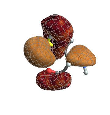 

Many thanks to Daniel Healion for the ReadCube and WriteCube functions.

Mathematica has enormous built-in capabilities to produce all sorts of data visualisations. Accessing that power can be tricky sometimes, though. And it often takes quite a bit of fiddling to produce the kinds of plots that certain disciplines consider to be appropriate for their field. Inspired by some recent posts, today I’m going to show how to construct different types of heat maps, and how to use Grid, instead of GraphicsGrid, to combine graphics more easily. more »

Mathematica has powerful graphics capabilities that can be used to explore the space of graphical forms in a very flexible way. Wolfram Research itself has already published a blog post showing how to manipulate various corporate logos, so it should be no surprise that the Mathematica StackExchange community came up with its own logo – not once, but twice! – and that we did it using Mathematica.

more »