Plotting electronic orbitals using Mathematica

2013-09-27 by . 8 comments

As a chemist it is often useful to plot electronic orbitals.  These are used to describe the wave function of electrons in atoms or molecules.  Typically, these are output from electronic structure software in the form of a cube file, first developed by Gaussian.  These files contain volumetric data for a given orbital on a three-dimensional grid.

There exist many applications to visualize cube files, such as VMD or GaussView, but I wanted to take advantage of Mathematica‘s  capability to easily combine graphics, as well as the ability to automate the process in order to efficiently create frames for a movie.

First off, we need a function to extract the data from the cube file.  In the process, we will create the text for an XYZ file, a format also developed by Gaussian.  The function OutForm is used here to mimic the printf function found in other programming languages.

OutForm[num_?NumericQ, width_Integer, ndig_Integer, 
   OptionsPattern[]] :=
  Module[{mant, exp, val},
   {mant, exp} = MantissaExponent[num];
   mant = ToString[NumberForm[mant, {ndig, ndig}]];
   exp = If[Sign[exp] == -1, "-", "+"] <> IntegerString[exp, 10, 2];
   val = mant <> "E" <> exp;
   StringJoin@PadLeft[Characters[val], width, " "]
   ];

ReadCube[cubeFileName_?StringQ] := Module[ {moltxt, nAtoms, lowerCorner, nx, ny, nz, xstep, ystep, zstep, atoms, desc1, desc2, xyzText, cubeDat, xgrid, ygrid, zgrid, dummy1, dummy2, atomicNumber, atomx, atomy, atomz, tmpString, headerTxt,bohr2angstrom}, bohr2angstrom = 0.529177249; moltxt = OpenRead[cubeFileName]; desc1 = Read[moltxt, String]; desc2 = Read[moltxt, String]; lowerCorner = {0, 0, 0}; {nAtoms, lowerCorner[[1]], lowerCorner[[2]], lowerCorner[[3]]} = Read[moltxt, String] // ImportString[#, "Table"][[1]] &; xyzText = ToString[nAtoms] <> "\n"; xyzText = xyzText <> desc1 <> desc2 <> "\n"; {nx, xstep, dummy1, dummy2} = Read[moltxt, String] // ImportString[#, "Table"][[1]] &; {ny, dummy1, ystep, dummy2} = Read[moltxt, String] // ImportString[#, "Table"][[1]] &; {nz, dummy1, dummy2, zstep} = Read[moltxt, String] // ImportString[#, "Table"][[1]] &; Do[ {atomicNumber, dummy1, atomx, atomy, atomz} = Read[moltxt, String] // ImportString[#, "Table"][[1]] &; xyzText = If[Sign[lowerCorner[[1]]] == 1, xyzText <> ElementData[atomicNumber, "Abbreviation"] <> OutForm[atomx, 17, 7] <> OutForm[atomy, 17, 7] <> OutForm[atomz, 17, 7] <> "\n", xyzText <> ElementData[atomicNumber, "Abbreviation"] <> OutForm[bohr2angstrom atomx, 17, 7] <> OutForm[bohr2angstrom atomy, 17, 7] <> OutForm[bohr2angstrom atomz, 17, 7] <> "\n"]; , {nAtoms}]; cubeDat = Partition[Partition[ReadList[moltxt, Number, nx ny nz], nz], ny]; Close[moltxt]; moltxt = OpenRead[cubeFileName]; headerTxt = Read[moltxt, Table[String, {2 + 4 + nAtoms}]]; Close[moltxt]; headerTxt = StringJoin@Riffle[headerTxt, "\n"]; xgrid = Range[lowerCorner[[1]], lowerCorner[[1]] + xstep (nx - 1), xstep]; ygrid = Range[lowerCorner[[2]], lowerCorner[[2]] + ystep (ny - 1), ystep]; zgrid = Range[lowerCorner[[3]], lowerCorner[[3]] + zstep (nz - 1), zstep]; {cubeDat, xgrid, ygrid, zgrid, xyzText, headerTxt} ];

If you need to create a cube file, then the following function can be used:
WriteCube[cubeFileName_?StringQ, headerTxt_?StringQ, cubeData_] := 
 Module[{stream}, 
  stream = OpenWrite[cubeFileName, FormatType -> FortranForm];
  WriteString[stream, headerTxt, "\n"];
  Map[WriteString[stream, ##, "\n"] & @@ 
     Riffle[ScientificForm[#, {3, 4}, 
         NumberFormat -> (Row[{#1, "E", If[#3 == "", "+00", #3], 
              "\t"}] &), NumberPadding -> {"", "0"}, 
         NumberSigns -> {"-", " "}] & /@ #, "\n", {7, -1, 7}] &, 
   cubeData, {2}];
  Close[stream];]
Next we need the function to plot the orbital,
CubePlot[{cub_, xg_, yg_, zg_, xyz_}, plotopts : OptionsPattern[]] := 
   Module[{xyzplot, bohr2picometer, datarange3D, pr},
    bohr2picometer = 52.9177249;
    datarange3D = 
      bohr2picometer {{xg[[1]], xg[[-1]]}, {yg[[1]], 
         yg[[-1]]}, {zg[[1]], zg[[-1]]}};
    xyzplot = ImportString[xyz, "XYZ"];
    Show[xyzplot, 
     ListContourPlot3D[Transpose[cub, {3, 2, 1}], 
       Evaluate[FilterRules[{plotopts}, Options[ListContourPlot3D]]], 
       Contours -> {-.02, .02}, ContourStyle -> {Blue, Red}, 
       DataRange -> datarange3D, MeshStyle -> Gray, 
       Lighting -> {{"Ambient", White}}], 
       Evaluate[
        FilterRules[{plotopts}, {ViewPoint, ViewVertical, ImageSize}]]]
    ];    
Let’s look at an example. Download the file cys-MO35.cube and place it in your home directory (or anywhere in your $Path). Then, read in the cube file with:
{cubedata,xg,yg,zg,xyz,header}= ReadCube["cys-MO35.cube"];
and plot it via
CubePlot[{cubedata, xg, yg, zg, xyz}]
pizCq

When I want to create a movie file, I want all the images to have exactly the same ViewAngle, ViewPoint, and ViewCenter.  When you give these options to CubePlot, it feeds them directly to the Show function

vp = {ViewCenter -> {0.5, 0.5, 0.5}, 
   ViewPoint -> {1.072, 0.665, -3.13}, 
   ViewVertical -> {0.443, 0.2477, 1.527}};

CubePlot[{cubedata, xg, yg, zg, xyz}, vp]

Q1mjs

Finally, you can also give any options that normally go to ListContourPlot3D

CubePlot[{cubedata, xg, yg, zg, xyz}, vp, 
 ContourStyle -> {Texture[ExampleData[{"ColorTexture", "Vavona"}]], 
   Texture[ExampleData[{"ColorTexture", "Amboyna"}]]}, 
 Contours -> {-.015, .015}] 
fLyJ7

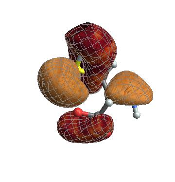
Many thanks to Daniel Healion for the ReadCube and WriteCube functions.

Filed under chemistry, graphics

Wolfram Technology Conference 2012

2012-10-29 by . 2 comments

The Wolfram Technology Conference took place from 2012-10-17 to 2012-10-19 in Champaign, IL. This is a loose collection of whatever interesting/entertaining stuff I came across during the conference. Note that I had to sign a non-disclosure agreement (NDA) to attend sessions on future Mathematica releases and upcoming Wolfram technology products, so there will be no infos on on that (make of that what you will).

Some general info for those who are not familiar with the Tech Conference:

There are several types of talks, and you can easily cram your schedule bumper to bumper:

  • WRI overview talks (presenting some topic, e.g. “Mathematica Connectivity” or “Image Processing” in general)
  • WRI in-depth talks (taking on a specific area, e.g. “Manipulate Secrets”)
  • Hands-on workshops (big this year: SystemModeler)
  • User talks that cover the wide range of Mathematica application in education, science, industry and entertainment. See the 2011 schedule and the 2012 videos to get an impression.

The Champaign Hilton Garden Inn is a decent venue, the only thing to be aware of is the sometimes lethal airconditioning, so be sure to bring warm clothes.

The focus of most presentations is on Mathematica, but since it is the Wolfram Technology Conference, things like Wolfram Alpha, SystemModeler and other technologies start to feature more and more prominently. There is an exceptional density of Wolfram developers (and thus WRI competence)  and you can set up meetings with them and other participants with the online conference system (crowdvine) or just try to taser and drag them into the coffee room downstairs (there is also a merchandise and book store offering conference discounts).

The program  is quite packed with three to four tracks and other things like meet-ups, lunch round tables on certain subjects and similar. On all evenings there is some kind social event either on-site or in Champaign at large. The crowd is a very easygoing one with a quite high proportion of regulars.

2012-10-15:

Landing at ORD.

Mathematica graphics

2012-10-16:

Yawn. The good thing about flying west is that getting up early (really early) is easy. Staying awake will be the hard part. Met Murta both in chat and real world  (see the chat transcript, and no, we did not make that up). Met up with rcollyer and a few WRI MMA.SE regulars at the reception.

2012-10-17:

Opening keynote by Stephen Wolfram: As every year, Stephen demoed a lot of interesting things to come — all of which were NDA’d. Bugger. Except for the fact that the next release will have version No. 9. Enjoyable: Stephen took the epic crashes of some demos (all on Apple devices) with good grace (John Fultz does not look too amused, though). Watch this:

Mathematica graphics

Accelerate session: One hour of 5min talks about things Mathematica. My personal highlight was Mark McClure’s astounding quadratic camera.  My 5min: a mashup of my selection of the most entertaining Q&A’s, most of them of the graphical persuasion:

Mathematica graphics

Stickers and pens provided by Aarthi vanished swiftly. It seems that Mathematica.SE is still not known to quite a number of serious Mathematica users.

2012-10-18:

Soundbite from the front end keynote by John Fultz about coming interface features (paraphrased): “We decided we needed more hubris, more arrogance. Stephen took the lead on that”.

Assembling all present MMA.SE personnel for the group shot proved astonishingly difficult (think herding cats), so this was the best one we got (From left to right: Mark McClure, Murta, rcollyer, Arnoud, Brett, myself, Michael Wijaya, Daniel ):

Mathematica graphics

Fun: “Connecting the ARDrone Quadrocopter to Mathematica” by Christopher Wolfram and Todd Gayley. The demo devil struck again, so for the first few minutes Todd did all the acting (including sound). Fear not, in the end the drone followed a simple line path defined in Mathematica and reacted to signs shown to it´s camera.

Mathematica graphics

Evening event: Conference Dinner. Food, drink and nice company and then Stephen presents the Wolfram Innovator Awards for the second time. I´ll not spoil the fun and tell and instead leave authoring the proper accolades to WRI on their blog. Check up on this year’s laureates. Not to be missed: The yearly comprehensive Q&A by Stephen.

Mathematica graphics

2012-10-19:

Shaky screenshot of my presentation, “Fun with Flaps”, which went reasonably well (well, it’s got airplanes in it and with that, plus pop culture reference, you cannot go wrong).

Mathematica graphics

Another really awful photo of one highly entertaining events: The oneliner competition. A pity that Chris Carlson’s hilarious presentation is not taped. Again, Chris will probably do a splendid job showing those oneliners on the Wolfram Blog, so I´ll simply mention that a certain CEO’s head featured prominently in the winner entry and then some. If you are not familiar with the oneliner competition, this one was the fourth (enjoy #1, #2 and #3).

Mathematica graphics

Remarkable: The youngest (conference, oneliner and probably Mathematica.SE) participant ever not related to WRI shareholders, Jesse Friedman, is eleven years old and got an honorable mention for his concise Wolfram Alpha interface oneliner which won him his own brandnew student license with upgrade to version 9! Kudos, Jesse! We are looking forward to hear more of you in the future.

Mathematica graphics

Nice:Luc Barthelet’s “Introduction to Image Processing–Solving the Rubik’s Cube from Pictures”

Mathematica graphics

One for the hardware-tinkerers: “Arduino and Mathematica – Computation in the Maker World”. A laser pointer controlled by an arduino board targets objects recognized by image processing in Mathematica.

Mathematica graphics

Evening Event: “Discover Downtown”: Free choice of several bars and restaurants in downtown Champaign, and coupons to redeem at will there (venue switching encouraged). From sushi to pizza, from sake to stout. One detail of one of the more robust venues in the murky birds-eye shot below:

Mathematica graphics

TL;DR

All in all, a really enjoyable, densely packed conference with excellent networking opportunities and highly recommended if you are a serious Mathematica user (or seriously planning on becoming one).

PS: Heavy loot from the oneliner competition: Generous WRI goodie basket! As far as carry-on luggage goes, this really makes one think about getting a kindle.

Mathematica graphics

PPS: Thanks to the Stackexchange team (esp. Aarthi) for providing swag and support! I still got some stickers, but t-shirts and pens sure diffused nicely.

Filed under uncategorized

What’s in, docs?

2012-10-08 by . 4 comments

After using Mathematica for a while, you start to think you are on top of the richness of the language. You become familiar with a range of different functions and programming styles. But in fact, you haven’t even scratched the surface.

I can’t emphasize enough how important it is to look up the documentation from time to time, even for the functions you think you already know. There are so many options and additional arguments to workhorse functions that you might not have appreciated. Here are a few of my favorites. Some of them were noted in a question I once asked about the issue.

Hooray for Array

If you want to iterate over arbitrary objects, you need Table.

Table[f[i], {i, {a, b, whatever}}]
{f[a], f[b], f[whatever]}

If instead the iterator increments by one each time, Array is cleaner. You don’t even need to give the iterator a name.

Array[f, 3]
{f[1], f[2], f[3]}

It’s easy to forget the extended forms of standard functions like this. The iterator in Array does not have to start at 1. Don’t forget that the first argument gives the resulting list’s length, not the end value of the iterator.

Array[f, {3}, {5}]
{f[5], f[6], f[7]}

This is a general example of the flexible pattern-matching in Mathematica, which allows separate function definitions for different numbers and types of arguments.

Totally rad

Total[somematrix, {2}] 

is equivalent to Mapping the Total function onto the rows of the matrix.

Partition magic

The third argument to Partition defines the offset, so that instead of

Partition[Array[f, 5], 2] // TableForm
f[1]    f[2]
f[3]    f[4]

You get

Partition[Array[f, 5], 2, 1] // TableForm
f[1]    f[2]
f[2]    f[3]
f[3]    f[4]
f[4]    f[5]

This means that, for example

Divide @@@ Partition[somevector, 2, 1] 

is equivalent to

Most[somevector]/Rest[somevector]

This question on the Mathematica.SE site shows how to generalise Partition for ragged lists (i.e., those with sub-lists that are not all the same length). There are a number of different ways to do this, including using Partition itself, as well as various combinations of NestWhile and Prepend.

Join in the fun

The third argument of Join is also incredibly useful. How many times have you seen complicated code with Transpose and Append all over the place, just to join two matrices by column, instead of by row? The default syntax for Join joins the rows, but you can join by columns with just two extra keystrokes. As noted in the answers to this question, this is also usually a little faster than the little-known but highly useful ArrayFlatten function.

Join[Array[g, {4, 2}], Array[f, {4, 2}]] // TableForm
g[1,1]  g[1,2]
g[2,1]  g[2,2]
g[3,1]  g[3,2]
g[4,1]  g[4,2]
f[1,1]  f[1,2]
f[2,1]  f[2,2]
f[3,1]  f[3,2]
f[4,1]  f[4,2]

Join[Array[g, {4, 2}], Array[f, {4, 2}], 2] // TableForm g[1,1] g[1,2] f[1,1] f[1,2] g[2,1] g[2,2] f[2,1] f[2,2] g[3,1] g[3,2] f[3,1] f[3,2] g[4,1] g[4,2] f[4,1] f[4,2]

Flip and Flatten

There are also additional options and arguments in some other basic list-manipulation commands. For example, most experienced users know that Flatten takes a level specification. For example, Flatten[list,1] turns a three-dimensional tensor into a matrix.

Flatten[Array[f, {3, 3, 2}], 1] // TableForm
f[1,1,1]    f[1,1,2]
f[1,2,1]    f[1,2,2]
f[1,3,1]    f[1,3,2]
f[2,1,1]    f[2,1,2]
f[2,2,1]    f[2,2,2]
f[2,3,1]    f[2,3,2]
f[3,1,1]    f[3,1,2]
f[3,2,1]    f[3,2,2]
f[3,3,1]    f[3,3,2]

But did you know that the second argument can also be a matrix? This popular question on the Mathematica.SE site contains a lot of information about how it works. It can be used to Transpose ragged lists, as this answer explains.

Speaking of Transpose, consider what is possible using its second argument. Here is the result of a normal transpose on a three-dimensional list with dimensions 342.

t1 = Transpose[Array[f, {3, 4, 2}]]
{{{f[1, 1, 1], f[1, 1, 2]}, {f[2, 1, 1], f[2, 1, 2]}, {f[3, 1, 1], f[3, 1, 2]}}, {{f[1, 2, 1], f[1, 2, 2]}, {f[2, 2, 1], f[2, 2, 2]}, {f[3, 2, 1], f[3, 2, 2]}}, {{f[1, 3, 1], f[1, 3, 2]}, {f[2, 3, 1], f[2, 3, 2]}, {f[3, 3, 1], f[3, 3, 2]}}, {{f[1, 4, 1], f[1, 4, 2]}, {f[2, 4, 1], f[2, 4, 2]}, {f[3, 4, 1], f[3, 4, 2]}}}

Effectively it treats the list as a matrix to transpose normally: it just happens that the elements of that matrix are themselves lists.

Dimensions@t1
{4, 3, 2}

You can get a completely different result by choosing a different specification in the second argument of Transpose. (The default is equivalent to specifying {2,1,3} for the second argument.)

t2 = Transpose[Array[f, {3, 4, 2}], {2, 3, 1}]
{{{f[1, 1, 1], f[1, 2, 1], f[1, 3, 1], f[1, 4, 1]}, {f[2, 1, 1], 
   f[2, 2, 1], f[2, 3, 1], f[2, 4, 1]}, {f[3, 1, 1], f[3, 2, 1], 
   f[3, 3, 1], f[3, 4, 1]}}, {{f[1, 1, 2], f[1, 2, 2], f[1, 3, 2], 
   f[1, 4, 2]}, {f[2, 1, 2], f[2, 2, 2], f[2, 3, 2], 
   f[2, 4, 2]}, {f[3, 1, 2], f[3, 2, 2], f[3, 3, 2], f[3, 4, 2]}}}

Dimensions@t2
{2, 3, 4}

The Bottom Line

Bottom line? Even if you are an experienced Mathematica user, it is worth having a good look at the documentation for basic functions from time to time. You might be missing some of the power they contain in their optional arguments.

Filed under programming

Turning up the Heat Maps

2012-10-01 by . 3 comments

Mathematica has enormous built-in capabilities to produce all sorts of data visualisations. Accessing that power can be tricky sometimes, though. And it often takes quite a bit of fiddling to produce the kinds of plots that certain disciplines consider to be appropriate for their field. Inspired by some recent posts, today I’m going to show how to construct different types of heat maps, and how to use Grid, instead of GraphicsGrid, to combine graphics more easily. more »

Filed under graphics

Build Your Own Logo with Mathematica (and a Few Friends)

2012-07-26 by . 4 comments

Mathematica has powerful graphics capabilities that can be used to explore the space of graphical forms in a very flexible way. Wolfram Research itself has already published a blog post showing how to manipulate various corporate logos, so it should be no surprise that the Mathematica StackExchange community came up with its own logo – not once, but twice! – and that we did it using Mathematica.

more »

Filed under graphics

Hello World!

2012-07-21 by . 0 comments

Welcome to the Mathematica Stack Exchange Q&A site’s blog! We are so excited to introduce the blog, to coincide with the graduation of the site itself.

We will have plenty to talk about, from behind-the-scenes explications of our most popular posts, to exposés on how to get even more out of the Mathematica software. Mathematica is an exceptionally rich environment that goes beyond pure programming. Over on the Q&A site, you will find questions (and answers) on front-end features like stylesheets, as well as interfacing with other languages, and everything in between. We also have some questions that are just plain fun!

As for who we are, the blog team is made up of many of the regular users on the Mathematica Stack Exchange site, including the moderators and some of the other top-ranking participants. Our backgrounds and expertise are diverse, but we’re all enthusiastic about the possibilities that Mathematica can offer.

Filed under uncategorized