![]()
As a chemist it is often useful to plot electronic orbitals. These are used to describe the wave function of electrons in atoms or molecules. Typically, these are output from electronic structure software in the form of a cube file, first developed by Gaussian. These files contain volumetric data for a given orbital on a three-dimensional grid.
There exist many applications to visualize cube files, such as VMD or GaussView, but I wanted to take advantage of Mathematica‘s capability to easily combine graphics, as well as the ability to automate the process in order to efficiently create frames for a movie.
First off, we need a function to extract the data from the cube file. In the process, we will create the text for an XYZ file, a format also developed by Gaussian. The function OutForm is used here to mimic the printf function found in other programming languages.
OutForm[num_?NumericQ, width_Integer, ndig_Integer,
   OptionsPattern[]] :=
  Module[{mant, exp, val},
   {mant, exp} = MantissaExponent[num];
   mant = ToString[NumberForm[mant, {ndig, ndig}]];
   exp = If[Sign[exp] == -1, "-", "+"] <> IntegerString[exp, 10, 2];
   val = mant <> "E" <> exp;
   StringJoin@PadLeft[Characters[val], width, " "]
   ];

ReadCube[cubeFileName_?StringQ] := Module[
   {moltxt, nAtoms, lowerCorner, nx, ny, nz, xstep, ystep, zstep,
    atoms, desc1, desc2, xyzText, cubeDat, xgrid, ygrid, zgrid,
    dummy1, dummy2, atomicNumber, atomx, atomy, atomz, tmpString,
    headerTxt,bohr2angstrom},
   bohr2angstrom = 0.529177249;
   moltxt = OpenRead[cubeFileName];
   desc1 = Read[moltxt, String];
   desc2 = Read[moltxt, String];
   lowerCorner = {0, 0, 0};
   {nAtoms, lowerCorner[[1]], lowerCorner[[2]], lowerCorner[[3]]} =
    Read[moltxt, String] // ImportString[#, "Table"][[1]] &;
   xyzText = ToString[nAtoms] <> "\n";
   xyzText = xyzText <> desc1 <> desc2 <> "\n";
   {nx, xstep, dummy1, dummy2} =
    Read[moltxt, String] // ImportString[#, "Table"][[1]] &;
   {ny, dummy1, ystep, dummy2} =
    Read[moltxt, String] // ImportString[#, "Table"][[1]] &;
   {nz, dummy1, dummy2, zstep} =
    Read[moltxt, String] // ImportString[#, "Table"][[1]] &;
   Do[
    {atomicNumber, dummy1, atomx, atomy, atomz} =
     Read[moltxt, String] // ImportString[#, "Table"][[1]] &;
    xyzText = If[Sign[lowerCorner[[1]]] == 1,
      xyzText <> ElementData[atomicNumber, "Abbreviation"] <>
       OutForm[atomx, 17, 7] <> OutForm[atomy, 17, 7] <>
       OutForm[atomz, 17, 7] <> "\n",
      xyzText <> ElementData[atomicNumber, "Abbreviation"] <>
       OutForm[bohr2angstrom atomx, 17, 7] <>
       OutForm[bohr2angstrom atomy, 17, 7] <>
       OutForm[bohr2angstrom atomz, 17, 7] <> "\n"];
    , {nAtoms}];
   cubeDat =
    Partition[Partition[ReadList[moltxt, Number, nx ny nz], nz], ny];
   Close[moltxt];
   moltxt = OpenRead[cubeFileName];
   headerTxt = Read[moltxt, Table[String, {2 + 4 + nAtoms}]];
   Close[moltxt];
   headerTxt = StringJoin@Riffle[headerTxt, "\n"];
   xgrid =
    Range[lowerCorner[[1]], lowerCorner[[1]] + xstep (nx - 1), xstep];
   ygrid =
    Range[lowerCorner[[2]], lowerCorner[[2]] + ystep (ny - 1), ystep];
   zgrid =
    Range[lowerCorner[[3]], lowerCorner[[3]] + zstep (nz - 1), zstep];
   {cubeDat, xgrid, ygrid, zgrid, xyzText, headerTxt}
   ];
WriteCube[cubeFileName_?StringQ, headerTxt_?StringQ, cubeData_] :=
 Module[{stream},
  stream = OpenWrite[cubeFileName, FormatType -> FortranForm];
  WriteString[stream, headerTxt, "\n"];
  Map[WriteString[stream, ##, "\n"] & @@
     Riffle[ScientificForm[#, {3, 4},
         NumberFormat -> (Row[{#1, "E", If[#3 == "", "+00", #3],
              "\t"}] &), NumberPadding -> {"", "0"},
         NumberSigns -> {"-", " "}] & /@ #, "\n", {7, -1, 7}] &,
   cubeData, {2}];
Close[stream];]CubePlot[{cub_, xg_, yg_, zg_, xyz_}, plotopts : OptionsPattern[]] :=
Module[{xyzplot, bohr2picometer, datarange3D, pr},
bohr2picometer = 52.9177249;
datarange3D =
bohr2picometer {{xg[[1]], xg[[-1]]}, {yg[[1]],
yg[[-1]]}, {zg[[1]], zg[[-1]]}};
xyzplot = ImportString[xyz, "XYZ"];
Show[xyzplot,
ListContourPlot3D[Transpose[cub, {3, 2, 1}],
Evaluate[FilterRules[{plotopts}, Options[ListContourPlot3D]]],
Contours -> {-.02, .02}, ContourStyle -> {Blue, Red},
DataRange -> datarange3D, MeshStyle -> Gray,
Lighting -> {{"Ambient", White}}],
Evaluate[
FilterRules[{plotopts}, {ViewPoint, ViewVertical, ImageSize}]]]
]; $Path). Then, read in the cube file with:
{cubedata,xg,yg,zg,xyz,header}= ReadCube["cys-MO35.cube"];CubePlot[{cubedata, xg, yg, zg, xyz}]
When I want to create a movie file, I want all the images to have exactly the same ViewAngle, ViewPoint, and ViewCenter. When you give these options to CubePlot, it feeds them directly to the Show function
vp = {ViewCenter -> {0.5, 0.5, 0.5},
   ViewPoint -> {1.072, 0.665, -3.13},
   ViewVertical -> {0.443, 0.2477, 1.527}};

CubePlot[{cubedata, xg, yg, zg, xyz}, vp]

Finally, you can also give any options that normally go to ListContourPlot3D
CubePlot[{cubedata, xg, yg, zg, xyz}, vp,
 ContourStyle -> {Texture[ExampleData[{"ColorTexture", "Vavona"}]],
   Texture[ExampleData[{"ColorTexture", "Amboyna"}]]},
Contours -> {-.015, .015}] 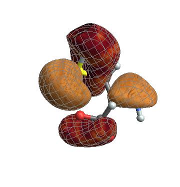
Many thanks to Daniel Healion for the ReadCube and WriteCube functions.
I never used Guassian, but Wien2k was my mainstay. I never considered posting the stuff I used for generating plots from it, though. Nice.
To anyone trying to work the example, for now you have to extract the archive yoursef, as Mathematica won’t extract it properly.
I tried to import the “cys-MO35cube” file extracted from the archive and placed in
$UserBaseDirectoryusing the{cubedata,xg,yg,zg,xyz,header}= ReadCube["cys-MO35.cube"];command and{cubedata,xg,yg,zg,xyz,header}= ReadCube["cys-MO35cube"];command but it fails. I am using MMa 8.0.4 under Win 7 x64. How it is supposed to work?Alexey, my apologies. The blog here keeps renaming my gzip archive, which then somehow renames the file inside the archive. So basically the extracted file doesn’t have the right filename. I’m very unfamiliar with the gzip format. I first tried to just upload the cube file in its uncompressed form, but the site has a size limit on uploads.
So I just fixed the link so that it points directly to the .cube file in my Dropbox folder. Let me know if you can make it work now.
Thank you, now it works. Very impressive! BTW, the file should be placed somewhere in
$Pathand$UserBaseDirectorywith$BaseDirectoryby default are not included in$Path. By default$HomeDirectoryis included, so it would be better to recommend users to place the file in this directory.Thanks for the help Alexey. I edited the post to be more clear.
Thanks Jason. Good basis for a tool I’m writing.
How would I go about counting the amount of lobes in the graphics you produce? Also perhaps the average size of the lobes / the localization of the lobes?
Thanks ahead of time.
Best wishes, Duhe